Note: This post was generated with AI tools for the sole purpose of demonstrating the rich typographic and mathematical capabilities of the Eyvan template.
Quantum entanglement represents one of the most important departures of quantum mechanics from the classical worldview. It changes how we think about physical reality, locality, measurement, and information. First brought into sharp focus by Einstein, Podolsky, and Rosen (EPR) in 1935 as part of an argument about the incompleteness of quantum theory, entanglement describes a non-separable state of a composite system: the whole system has a well-defined quantum state, but its parts cannot always be assigned independent pure states.
Decades later, John Stewart Bell transformed the EPR debate from a philosophical question into an experimentally testable one. Bell showed that any theory satisfying local realism must obey statistical constraints known as Bell inequalities. Quantum mechanics predicts that entangled systems can violate those constraints. Later experiments confirmed these violations, making entanglement not merely a conceptual puzzle but a practical resource for quantum computation, quantum cryptography, quantum communication, and quantum metrology.
This primer introduces the basic formalism of bipartite entanglement, the density matrix description of local subsystems, the CHSH form of Bell’s inequality, and the experimental logic behind modern Bell tests.
Historical Context and Non-Separability
The intellectual origin of entanglement is closely tied to the EPR paradox. EPR argued that if local realism were true, quantum mechanics must be incomplete. Here, realism means that physical systems possess definite properties independent of measurement, while locality means that actions performed at one location cannot instantly affect a distant physical system.
EPR used a highly correlated bipartite state to argue that distant measurements seemed to reveal pre-existing “elements of reality.” Shortly afterward, Erwin Schrödinger recognized the deeper implication of the wave function and introduced the term Verschränkung, or entanglement, for situations in which the state of the whole cannot be reduced to independent states of the parts.
Mathematically, consider a composite Hilbert space
\[\mathcal{H} = \mathcal{H}_A \otimes \mathcal{H}_B,\]
where subsystem $A$ is held by Alice and subsystem $B$ is held by Bob. A pure state $\ket{\psi} \in \mathcal{H}$ is called separable if it can be written as a tensor product of two subsystem states:
\[\ket{\psi} = \ket{\phi}_A \otimes \ket{\chi}_B.\]
A state is entangled if it cannot be written in this product form.
A standard example of a maximally entangled two-qubit state is the Bell state
\[\ket{\Phi^+} = \frac{1}{\sqrt{2}}(\ket{00} + \ket{11}).\]
Another important Bell state is the singlet state,
\[\ket{\Psi^-} = \frac{1}{\sqrt{2}}(\ket{01} - \ket{10}),\]
which is especially useful in spin and polarization discussions because its correlations are rotationally invariant. Both states are maximally entangled, but their correlation functions differ by signs and basis conventions. Keeping these states distinct is important when deriving Bell-inequality violations.
Visualizing Entanglement vs. Classical Correlation
A helpful way to understand the difference between entanglement and classical correlation is to compare how each behaves under changes of measurement basis. Photon polarization experiments are especially useful for this purpose.
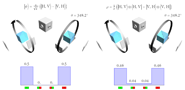
Side-by-side simulation demonstrating the operational difference between a maximally entangled singlet state and a dephased, classically correlated mixed state. Source: Wikimedia Commons, creator JozumBjada, November 27, 2020, licensed under Creative Commons CC BY-SA 4.0.
The visualization compares two situations:
- Entangled pair: the photons are described by a coherent joint quantum state.
- Classically correlated pair: the photons are correlated in the horizontal/vertical basis, but the quantum coherence between alternatives has been removed.
In both scenes, a central source emits photon pairs. One photon travels to Alice’s measurement station and the other travels to Bob’s. Each station contains a polarization analyzer and detectors. When both analyzers measure in the same horizontal/vertical basis, the entangled state and the classically correlated mixed state can produce similar-looking statistics. This is why a single measurement basis is not enough to demonstrate entanglement.
The difference appears when the measurement bases are rotated. For the singlet state, the correlations depend only on the relative angle between Alice’s and Bob’s measurement bases, not on their shared absolute orientation. By contrast, the dephased classically correlated state retains a preferred horizontal/vertical basis, so its statistics change under common rotations of the analyzers.
This is one of the key operational differences between quantum entanglement and classical correlation: entanglement is not simply “very strong correlation.” It is correlation carried by a coherent joint state that cannot be represented as a classical mixture of independent local properties.
State vectors are sufficient for describing isolated pure states, but they are not enough when we want to describe mixed states or local subsystems of an entangled pair. For that, we use the density matrix formalism.
For a pure state $\ket{\psi}$, the global density operator is
\[\rho = \ket{\psi}\bra{\psi}.\]
To determine the state accessible to Alice alone, we trace over Bob’s subsystem. This operation is called the partial trace:
\[\rho_A = \operatorname{Tr}_B(\rho)
= \sum_i
(\mathbb{I}_A \otimes \bra{i}_B)
\rho
(\mathbb{I}_A \otimes \ket{i}_B).\]
Apply this to the Bell state
\[\ket{\Phi^+} = \frac{1}{\sqrt{2}}(\ket{00} + \ket{11}).\]
The global density matrix is
\[\rho =
\ket{\Phi^+}\bra{\Phi^+}
=
\frac{1}{2}
\Big(
\ket{00}\bra{00}
+
\ket{00}\bra{11}
+
\ket{11}\bra{00}
+
\ket{11}\bra{11}
\Big).\]
Taking the partial trace over Bob’s qubit gives Alice’s reduced density matrix:
\[\rho_A
=
\operatorname{Tr}_B(\rho)
=
\frac{1}{2}
\Big(
\ket{0}\bra{0}
+
\ket{1}\bra{1}
\Big)
=
\frac{1}{2}\mathbb{I}_A.\]
This result is important. The global state $\rho$ is pure, with zero von Neumann entropy,
\[S(\rho) = -\operatorname{Tr}(\rho \log \rho) = 0.\]
But Alice’s local state is maximally mixed:
\[S(\rho_A) = \log 2.\]
Alice sees locally random outcomes, even though the two-qubit system as a whole is in a pure coherent state. This contrast between global purity and local mixedness is one of the formal signatures of entanglement.
Bell’s Theorem and the CHSH Inequality
For nearly three decades after EPR, the debate about locality and realism remained largely conceptual. Bell changed this in 1964 by showing that local hidden-variable theories obey experimentally testable constraints. These constraints are now called Bell inequalities.
The most commonly discussed version is the Clauser-Horne-Shimony-Holt, or CHSH, inequality.
Suppose Alice can choose between two dichotomic observables, $A$ and $A’$, each producing outcomes in ${+1, -1}$. Bob can choose between two observables, $B$ and $B’$, also producing outcomes in ${+1, -1}$. Let $E(A,B)$ be the expectation value of the product of Alice’s and Bob’s outcomes for a given pair of settings.
Under local realism, the CHSH expression must satisfy
\[\left|
E(A,B)
+
E(A,B')
+
E(A',B)
-
E(A',B')
\right|
\leq 2.\]
The upper bound of $2$ is not a limitation of a particular apparatus. It follows from the assumptions that measurement outcomes are locally determined and that the choice of measurement setting at one site does not influence the outcome at the other site.
Quantum mechanics predicts that entangled states can violate this bound. The maximum quantum value is
\[2\sqrt{2} \approx 2.828,\]
known as Tsirelson’s bound.
Walkthrough Derivation of CHSH Violation
To see how the violation appears mathematically, we can use the Bell state $\ket{\Phi^+}$ and restrict all measurement directions to the $x$-$z$ plane.
Alice and Bob share
\[\ket{\Phi^+} =
\frac{1}{\sqrt{2}}(\ket{00} + \ket{11}).\]
Alice chooses between two measurement directions, represented by unit vectors $\vec{a}$ and $\vec{a}’$. Bob chooses between $\vec{b}$ and $\vec{b}’$. The corresponding observables are
\[A = \vec{a}\cdot\vec{\sigma},
\qquad
B = \vec{b}\cdot\vec{\sigma},\]
where $\vec{\sigma}$ denotes the vector of Pauli matrices.
For this state and this measurement plane, the quantum correlation function is
\[E(\vec{a},\vec{b})
=
\bra{\Phi^+}
(\vec{a}\cdot\vec{\sigma})
\otimes
(\vec{b}\cdot\vec{\sigma})
\ket{\Phi^+}
=
\vec{a}\cdot\vec{b}
=
\cos(\theta_{\vec{a},\vec{b}}),\]
where $\theta_{\vec{a},\vec{b}}$ is the angle between the two measurement directions.
Choose the following settings:
- Alice’s first setting: $\theta_A = 0^\circ$
- Alice’s second setting: $\theta_{A’} = 90^\circ$
- Bob’s first setting: $\theta_B = 45^\circ$
- Bob’s second setting: $\theta_{B’} = -45^\circ$
Using
\[E(\vec{a},\vec{b}) = \cos(\Delta \theta),\]
we get
\[E(A,B) = \cos(45^\circ - 0^\circ) = \frac{\sqrt{2}}{2},\]
\[E(A,B') = \cos(-45^\circ - 0^\circ) = \frac{\sqrt{2}}{2},\]
\[E(A',B) = \cos(45^\circ - 90^\circ) = \frac{\sqrt{2}}{2},\]
and
\[E(A',B') = \cos(-45^\circ - 90^\circ) = -\frac{\sqrt{2}}{2}.\]
Substitute these values into the CHSH expression:
\[S =
E(A,B)
+
E(A,B')
+
E(A',B)
-
E(A',B').\]
Then
\[S =
\frac{\sqrt{2}}{2}
+
\frac{\sqrt{2}}{2}
+
\frac{\sqrt{2}}{2}
-
\left(
-\frac{\sqrt{2}}{2}
\right)
=
2\sqrt{2}.\]
Because
\[2\sqrt{2} > 2,\]
the quantum prediction violates the CHSH inequality. This means that no local hidden-variable theory satisfying the CHSH assumptions can reproduce all the statistical predictions of quantum mechanics.
If the singlet state $\ket{\Psi^-}$ is used instead, the correlation function becomes
\[E(\vec{a},\vec{b}) = -\vec{a}\cdot\vec{b}.\]
The sign convention changes, but with appropriate measurement settings the same maximum violation magnitude, $2\sqrt{2}$, is obtained.
Summary of Empirical Milestones
Bell-test experiments attempt to determine whether observed correlations can be explained by local hidden variables or whether they violate Bell inequalities as quantum mechanics predicts.
The main experimental challenge is closing loopholes. The classic loopholes include:
- Locality loophole: the possibility that information about one measurement setting or outcome reaches the other detector in time to influence the result.
- Detection loophole: the possibility that the detected subset of particles is not representative of the full emitted ensemble.
- Freedom-of-choice loophole: the possibility that the measurement settings are not statistically independent of hidden variables associated with the source.
The following table summarizes selected milestones.
Selected experimental milestones in Bell-test verification and loophole closure.
| Experiment / Laboratory |
Physical System |
Reported Bell-test result |
Statistical Confidence |
Main Loophole Addressed |
| Freedman & Clauser (1972) |
Atomic calcium cascade photons |
Bell-inequality violation observed |
Significant early violation |
First widely recognized experimental Bell test |
| Aspect, Dalibard & Roger (1982) |
Entangled photons |
Bell-inequality violation with time-varying analyzers |
Strong violation |
Locality through fast analyzer switching |
| Rowe et al. (2001) |
Trapped $^{9}\mathrm{Be}^{+}$ ions |
Bell-type violation using high-efficiency ion detection |
Strong violation |
Detection efficiency |
| Hensen et al. (Delft, 2015) |
Nitrogen-vacancy centers in diamond |
$S = 2.42 \pm 0.20$ |
$p = 0.039$ |
Loophole-free test addressing locality and detection |
| Giustina et al. (Vienna, 2015) |
Entangled photons |
Significant Bell-inequality violation |
$11.5\sigma$ |
Loophole-free photonic test with high-efficiency detection |
| Shalm et al. (NIST, 2015) |
Entangled photons from spontaneous parametric down-conversion |
Significant Bell-inequality violation |
Strong rejection of local realism |
Loophole-free photonic test with high spatial separation |
These experiments do not prove that measurement outcomes are controlled by faster-than-light signals. Rather, they show that the joint assumptions of locality, realism, and standard statistical independence cannot all be maintained in the simple classical form assumed by local hidden-variable models.
Reproducibility and Numerical Verification
The CHSH violation can be verified numerically with basic matrix algebra. Define the Pauli matrices
\[\sigma_x =
\begin{pmatrix}
0 & 1 \\
1 & 0
\end{pmatrix},
\qquad
\sigma_z =
\begin{pmatrix}
1 & 0 \\
0 & -1
\end{pmatrix}.\]
A measurement direction in the $x$-$z$ plane can be represented as
\[\sigma(\theta)
=
\sin(\theta)\sigma_x
+
\cos(\theta)\sigma_z.\]
For two qubits, the joint observable is built using the tensor product:
\[\sigma(\theta_A) \otimes \sigma(\theta_B).\]
The correlation is then computed as
\[E(\theta_A,\theta_B)
=
\bra{\Phi^+}
\left[
\sigma(\theta_A) \otimes \sigma(\theta_B)
\right]
\ket{\Phi^+}.\]
By evaluating this expression for the four CHSH settings,
\[\theta_A = 0^\circ,
\qquad
\theta_{A'} = 90^\circ,
\qquad
\theta_B = 45^\circ,
\qquad
\theta_{B'} = -45^\circ,\]
one recovers
\[S = 2\sqrt{2}.\]
This computation is straightforward to reproduce in Python with NumPy using Kronecker products. Conceptually, it shows that the violation is not an artifact of language or interpretation; it follows from the linear algebraic structure of quantum states and measurements.
Conclusion
Entanglement is not merely a stronger version of classical correlation. It is a structural feature of composite quantum systems whose joint state cannot be decomposed into independent local states. The density matrix formalism shows how a globally pure state can produce locally mixed subsystems, while Bell’s theorem shows that entangled states can generate correlations beyond the limits of local hidden-variable theories.
The CHSH inequality makes this distinction experimentally testable. Its violation demonstrates that the classical assumptions of locality, realism, and independent measurement choice cannot all be retained in their traditional form. This is why entanglement remains central not only to the foundations of quantum mechanics, but also to modern quantum technologies.
References
- Aspect, A., Dalibard, J., & Roger, G. (1982). Experimental test of Bell’s inequalities using time-varying analyzers. Physical Review Letters, 49(25), 1804–1807.
- Bell, J. S. (1964). On the Einstein Podolsky Rosen paradox. Physics Physique Fizika, 1(3), 195–200.
- Clauser, J. F., Horne, M. A., Shimony, R., & Holt, R. A. (1969). Proposed experiment to test local hidden-variable theories. Physical Review Letters, 23(15), 880–884.
- Einstein, A., Podolsky, B., & Rosen, N. (1935). Can quantum-mechanical description of physical reality be considered complete? Physical Review, 47(10), 777–780.
- Freedman, S. J., & Clauser, J. F. (1972). Experimental test of local hidden-variable theories. Physical Review Letters, 28(14), 938–941.
- Giustina, M., et al. (2015). Significant-loophole-free test of Bell’s theorem with entangled photons. Physical Review Letters, 115(25), 250401.
- Hensen, B., et al. (2015). Loophole-free Bell inequality violation using electron spins separated by 1.3 kilometres. Nature, 526(7575), 682–686.
- Rowe, M. A., et al. (2001). Experimental violation of a Bell’s inequality with efficient detection. Nature, 409, 791–794.
- Shalm, L. K., et al. (2015). Strong loophole-free test of local realism. Physical Review Letters, 115(25), 250402.
Endnotes