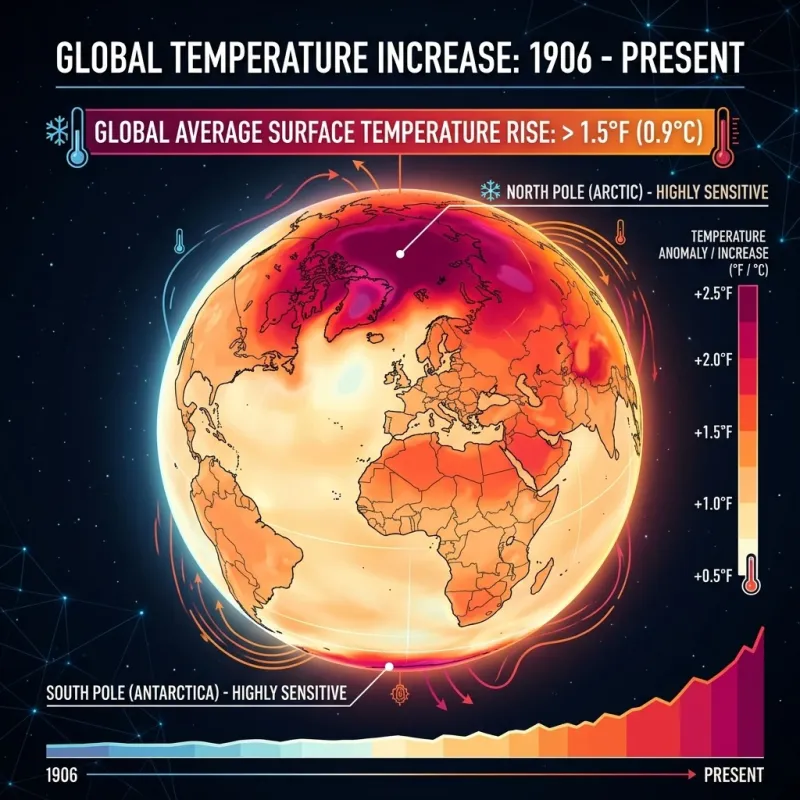
Note: This post and its associated synthetic, NOAA-inspired climate dataset were generated with AI tools to demonstrate Eyvan’s typography, mathematical notation, table captions, cross-references, and embedded charts. The values are plausible but should not be treated as a reproducible NOAA analysis unless they are replaced with a documented data pipeline and source files.
Template note: The interactive charts and demo-climate-charts.js are
demonstration content, not a core Eyvan dependency. Template users who do
not keep this post can remove the demo script with it.
Introduction & Methodology
The study of climate change benefits from clear analytical frameworks, especially when long-term trends need to be communicated through tables, figures, and statistical summaries. This demo post uses climate-style data to show how the Eyvan template handles mathematical notation, styled Markdown tables, numbered captions, cross-references, and embedded JavaScript charts.
The dataset below spans exactly 30 years, from 1996 through 2025. It is a synthetic, NOAA-inspired demonstration dataset rather than a directly downloaded observational record. The values are structured to resemble a regional mid-latitude climate summary, with yearly maximum temperature, minimum temperature, temperature anomaly, precipitation total, and precipitation-status fields.
Data Harmonization and Processing
Real climate datasets often require careful preprocessing before analysis. Station moves, changing instruments, missing values, observation-time differences, and urbanization effects can all influence raw measurements. A production-quality analysis should document the data source, processing scripts, quality-control decisions, and uncertainty assumptions.
For this template demonstration, the preprocessing steps are presented as representative examples rather than as operations actually performed on raw NOAA files:
- Time-of-observation adjustment: A real workflow may standardize daily readings to reduce artifacts introduced by morning or afternoon station resets.
- Homogenization: A real workflow may compare neighboring stations to identify artificial step changes caused by station relocation or equipment changes.
- Missing-value handling: A real workflow may flag, remove, or estimate missing observations depending on the amount of missingness and the research question.
The synthetic dataset is grouped into three distinct decadal epochs: Epoch I (1996–2005), Epoch II (2006–2015), and Epoch III (2016–2025). Segmenting the 30-year span into ten-year blocks helps demonstrate how tables and charts can communicate changes in central tendency and variability.
To establish a mathematical foundation for our observations, we employ standard descriptive statistics. When evaluating climate parameters over multi-decade intervals, tracking the shift in the central tendency alone is insufficient; we must also quantify the dispersion and volatility of these systems.
The arithmetic mean ($\bar{x}$) represents the foundational baseline for decadal averages, calculated as:
\[\bar{x} = \frac{1}{n}\sum_{i=1}^{n} x_i\]
Where $x_i$ denotes an individual annual or seasonal temperature/precipitation metric, and $n$ represents the total number of observed periods within that specific decade ($n = 10$ for annual aggregations within an epoch).
To measure the overall volatility and spread of temperatures within each epoch, we compute the sample standard deviation ($s$):
\[s = \sqrt{\frac{1}{n-1}\sum_{i=1}^{n} (x_i - \bar{x})^2}\]
A rising standard deviation over successive epochs would indicate increasing variability within the measured series. In this synthetic example, it is used to demonstrate how a post can discuss dispersion alongside changes in the mean.
Decadal Summary Statistics
Applying these formulas to the synthetic dataset yields a distinct trajectory. The table below presents aggregate summary metrics for surface temperatures across the three designated decades. Here, mean temperature corresponds to $\bar{x}$, standard deviation corresponds to $s$, and heat days count average annual days above $35$°C.
Synthetic decadal summary statistics for surface temperatures and extreme heat days.
| Epoch |
Time Period |
Mean Temp (°C) |
Median Temp (°C) |
Std Dev (°C) |
Heat Days >35°C |
| Epoch I |
1996–2005 |
14.21 |
14.15 |
0.62 |
12.4 |
| Epoch II |
2006–2015 |
14.68 |
14.52 |
0.78 |
18.1 |
| Epoch III |
2016–2025 |
15.14 |
15.11 |
0.94 |
24.5 |
Analysis of Decadal Summaries
The table reveals a clear upward shift in the synthetic central tendency metrics. The arithmetic mean ($\bar{x}$) rises by $0.47$°C between Epoch I and Epoch II, followed by an additional increase of $0.46$°C moving into Epoch III. This yields a net increase of $+0.93$°C over the 30-year demo period.
Concurrently, the sample standard deviation ($s$) expands from $0.62$°C to $0.94$°C. In a real observational study, that change would require uncertainty analysis before being interpreted as a robust increase in climate variability. In this demo dataset, it illustrates how Eyvan can present both central tendency and dispersion. The final column also demonstrates how derived metrics can be summarized: average annual heat days above $35$°C increase from $12.4$ days per year in Epoch I to $24.5$ days per year in Epoch III.
Comprehensive Annual Climate Record
To observe how these multi-decadal shifts appear on an annual basis, we can inspect the unaggregated demo series. The following multi-column table presents yearly temperature and precipitation values, including a synthetic temperature anomaly field modeled as if it were relative to a long-term baseline.
Synthetic annual temperature anomalies, precipitation totals, and climate variations from 1996 to 2025.
| Year |
Mean Max (°C) |
Mean Min (°C) |
Temp Anomaly (°C) |
Annual Precip (mm) |
Precip Status |
| 1996 |
19.4 |
8.8 |
-0.12 |
845 |
Normal |
| 1997 |
19.6 |
9.1 |
+0.05 |
892 |
Above Average |
| 1998 |
20.1 |
9.7 |
+0.41 |
780 |
Below Average |
| 1999 |
19.5 |
8.9 |
-0.03 |
830 |
Normal |
| 2000 |
19.3 |
8.7 |
-0.15 |
865 |
Normal |
| 2001 |
19.8 |
9.2 |
+0.18 |
812 |
Normal |
| 2002 |
19.9 |
9.4 |
+0.22 |
795 |
Below Average |
| 2003 |
20.2 |
9.6 |
+0.39 |
850 |
Normal |
| 2004 |
19.5 |
8.9 |
-0.01 |
910 |
Above Average |
| 2005 |
20.4 |
9.9 |
+0.51 |
824 |
Normal |
| 2006 |
20.5 |
10.1 |
+0.58 |
801 |
Normal |
| 2007 |
20.3 |
9.8 |
+0.44 |
742 |
Deficit |
| 2008 |
20.0 |
9.5 |
+0.21 |
885 |
Normal |
| 2009 |
20.2 |
9.6 |
+0.32 |
920 |
Above Average |
| 2010 |
20.8 |
10.4 |
+0.74 |
860 |
Normal |
| 2011 |
20.6 |
10.2 |
+0.61 |
955 |
Surge |
| 2012 |
21.2 |
10.9 |
+1.02 |
698 |
Severe Deficit |
| 2013 |
20.4 |
9.9 |
+0.49 |
872 |
Normal |
| 2014 |
20.7 |
10.3 |
+0.68 |
841 |
Normal |
| 2015 |
21.1 |
10.8 |
+0.95 |
815 |
Normal |
| 2016 |
21.4 |
11.1 |
+1.15 |
790 |
Below Average |
| 2017 |
21.3 |
11.0 |
+1.08 |
934 |
Above Average |
| 2018 |
21.6 |
11.4 |
+1.28 |
982 |
Surge |
| 2019 |
21.5 |
11.2 |
+1.19 |
804 |
Normal |
| 2020 |
21.9 |
11.8 |
+1.44 |
710 |
Deficit |
| 2021 |
21.7 |
11.5 |
+1.32 |
866 |
Normal |
| 2022 |
22.1 |
12.0 |
+1.56 |
1015 |
Extreme Surge |
| 2023 |
22.4 |
12.3 |
+1.78 |
650 |
Extreme Deficit |
| 2024 |
22.2 |
12.1 |
+1.62 |
890 |
Normal |
| 2025 |
22.6 |
12.5 |
+1.85 |
765 |
Below Average |
Interpretation of Year-over-Year Dynamics
Reviewing the annual records in tbl-annual-climate-record shows how a long table can support detailed interpretation. Early demo years such as 1996 and 2000 contain negative temperature anomalies, while the synthetic series contains only positive anomalies after 2010.
The year 2012 is the first year in this demo table where the temperature anomaly crosses the $+1.0$°C threshold ($+1.02$°C), coinciding with a low precipitation total ($698$ mm). This does not prove a causal relationship, but it illustrates how a post can connect tabular evidence to a cautious interpretation. The final five years show the highest values in the synthetic anomaly series, ending with $+1.85$°C in 2025.
Visualizing Temperature Trends
To translate the tabular record into an interpretable visual sequence, the interactive line chart below charts the progression of both mean maximum and mean minimum temperatures over the 30-year demo period.
Synthetic mean maximum and minimum surface temperature trajectories from 1996 to 2025.
Analysis of the Line Chart Trajectory
In this synthetic dataset, minimum temperatures rise faster than maximum temperatures. The mean maximum temperature increases from $19.4$°C in 1996 to $22.6$°C in 2025, while the mean minimum temperature increases from $8.8$°C to $12.5$°C over the same period.
This pattern is scientifically plausible: observed warming often affects nighttime minimum temperatures strongly because greenhouse gases reduce outgoing longwave cooling. However, the chart should be read as a demonstration of the template’s charting and caption system, not as evidence from a documented observational pipeline.
Hydrological Instability: Precipitation Volatility
While the synthetic temperature metrics follow a steady upward trajectory, precipitation behaves differently. Rather than showing a clean linear increase or decrease, the demo series alternates between wetter and drier years.
The bar chart below shows annual precipitation values, organized into three decadal blocks to illustrate variability across the demo period.
Synthetic annual precipitation variability grouped by decadal epoch from 1996 to 2025.
Interpretation of Hydrological Trends
The distribution of precipitation across the three epochs demonstrates how Eyvan handles a second chart type and a longer explanatory section. In Epoch I, precipitation remains within a relatively narrow range between $780$ mm and $910$ mm.
In Epoch II, the synthetic series becomes more variable, with a low value of $698$ mm in 2012 and a high value of $955$ mm in 2011. Epoch III contains the highest and lowest precipitation values in the demo table: $1015$ mm in 2022 and $650$ mm in 2023.
This pattern is consistent with a common climate-science explanation: a warmer atmosphere can hold more water vapor, approximately 7% more per 1°C of warming under Clausius-Clapeyron scaling. That physical relationship can contribute to heavier precipitation events in some contexts while also intensifying drying between storms. In this post, however, the precipitation sequence is illustrative rather than a formal statistical test.
Limitations & Caveats
Because this is a synthetic demo post, the main limitation is that the values are not reproducible observational results. A real analysis should include downloadable data, source URLs or DOIs, processing scripts, versioned dependencies, and documented quality-control decisions.
Additional limitations that would matter in a real climate-data workflow include:
- Spatial aggregation constraints: Regional averages can hide local variation and should define the included stations or grid cells.
- Urban heat island artifacts: Stations near expanding built environments may require careful treatment.
- Precipitation capture efficiency: Gauges can under-report precipitation during high winds or intense events.
- Uncertainty and significance: Trends should be tested statistically rather than inferred visually from a short table.
References
-
National Oceanic and Atmospheric Administration, Global Historical Climatology Network Daily (GHCN-Daily), Version 4.0, National Centers for Environmental Information, U.S. Department of Commerce (2025).
-
Intergovernmental Panel on Climate Change, Climate Change 2021: The Physical Science Basis, Contribution of Working Group I to the Sixth Assessment Report of the Intergovernmental Panel on Climate Change, Cambridge University Press, Cambridge, England (2021).
-
K. E. Trenberth, “Changes in precipitation with climate change,” Climate Research 47, 123–138 (2011).
Endnotes